The Data You Don’t Have

Where is the value in data science?

Phil Henrickson, PhD
Data Scientist
AE Business Solutions

Background

“For a decade now, [the role of] Data Scientist has been in the spotlight. AI experts had salaries that rivaled those of sports superstars.

In the search for fame and fortune, hundreds of young professionals entered into what seemed a frenetic golden rush… Whole new industries sprang around the hype.

Consulting specialists promised millions if your company could unlock the potential of data.

AI, or Machine Learning, has been called the new electricity and data, the new oil.”¹

1. Source: Matheus Facure, Causal Inference for the Brave and True

But there’s a problem.

Is all of this investment in data science actually worth anything?

Most organizations want to advance their capabilities in DS/ML/AI.

At the same time, most organizations struggle to find value from them.

In my humble estimation, I think this is because they are looking for value in the wrong places.

“During all of this time…

• economists were trying to answer what is the true impact of education on one’s earnings

• biostatisticians were trying to understand if saturated fat led to a higher chance of a heart attack

• psychologists were trying to understand if words of affirmation led indeed to a happier marriage.

We forgot about those who have been doing “old-fashioned” science with data all along.”¹

1. Source: Matheus Facure, Causal Inference for the Brave and True

What, really, is the value of data science?

The value of data science is simply that of science - it is the process by which we try to understand the world around us.

It allows us to discover cause and effect; it allows us to measure things we care about. It helps us understand the data we have and the data that we don’t.

To illustrate, I want to tell you two stories of “old fashioned” data science in action.

These stories involve two very different, yet related topics.

The second story is about an important topic that affects us all, something that weighs on us everyday and affects the physical well-being of ourselves and our loved ones: college football.

The first story is about heart disease.

1) What causes cardiovascular failure?

Have you ever gone to the doctor and received your ten-year cardiovascular risk score?

Have you ever wondered where that score comes from?

Would you have guessed that it had something to do with Franklin Delano Roosevelt?

President Roosevelt died on April 12, 1945, at the age of 63, from cerebral hemorrhage with a blood pressure of 300/190 mmHg.

By the 1940s, cardiovascular disease had become the number one cause of mortality among Americans, accounting for 1 in 2 deaths.

At this time, almost nothing was known about the causes of heart failure.

Prevention and treatment were so poorly understood that most Americans accepted early death from heart disease as unavoidable.

For example:

In 1932, candidate Roosevelt’s campaign office released medical records showing his blood pressure to be 140/100 mmHg, which did not prompt any medical intervention.

By 1941, the President experienced a gradual rise in blood pressure to 188/105 mmHg.

In March 1944, Dr. Bruenn noted that the patient appeared “slightly cyanotic” with blood pressure of 186/108 mmHg.

A month after coming under Dr. Bruenn’s care, Roosevelt’s blood pressure had risen to 240/130 mmHg.

FDR’s death in April of 1945 prompted a national call for the study of cardiovascular disease.

FDR’s death in April of 1945 prompted a national call for the study of cardiovascular disease.

On June 16, 1948, President Harry Truman signed into law the National Heart Act. This law approved a twenty-year epidemiological heart study and established the National Heart Institute.

This study was the brainchild of Joseph Mountin, a physician from Hartford, Wisconsin.

How do you determine the causes of long term heart risk?

Joseph Mountin recognized that the problem demanded a long term study; collecting the necessary data.

“Observations of population characteristics must be made well before disease becomes overt if the relationship of these characteristics to the development of the disease is to be established with reasonable certainty.”

How do you determine the causes of long term heart risk?

• Study a large group of people over a long period of time who have not yet developed overt symptoms of cardiovascular disease.

• Collect data on every individual at the start of the study and during regularly scheduled follow-ups.

• Observe them. Eventually, some of the individuals will experience cardiovascular disease.

• Examine the relationship between data collected at the beginning of the study and the onset of the disease.

So that is what they decided to do.

The town of Framingham, Massachusetts was chosen as the location for the study.

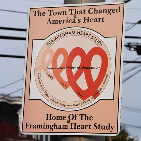
So that is what they decided to do.

The town of Framingham, Massachusetts was chosen as the location for the study.

The one-time farming community was now a factory town of 28,000 middle-class residents of predominantly European origin… and was “therefore considered to be representative of the United States in the 1940s”.

The original cohort was recruited between 1948 and 1952 and consisted of 5209 residents aged 28 to 62 years. Women comprised more than half of the participants in the study. The study’s inclusion of women contrasted with contemporaneous epidemiological studies, which had very small numbers of women or excluded them altogether.

What data did they choose to collect?

A committee of specialists had to speculate about the potential causes and develop a variety of hypotheses to guide their data collection.

They cast a pretty wide net in collecting data on individuals.

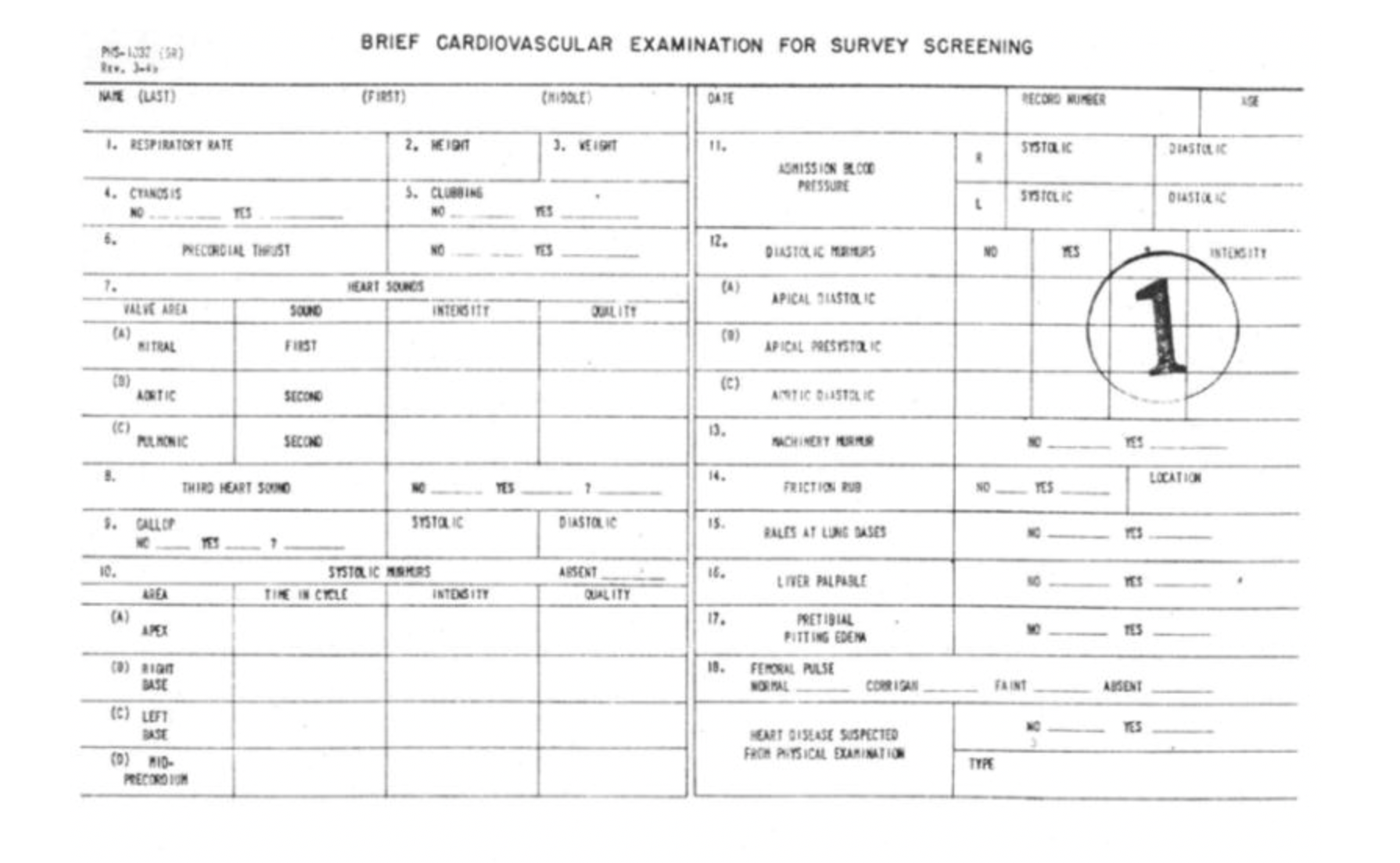
I requested the (anonymized) data from the Framingham study for the purpose of this talk.

This is a portion of the clinical data they collected.

sex	totchol	age	sysbp	diabp	smoker	bmi	heartrte	glucose	ten_year_chd
male	301	58	170.0	96.0	0	27.69	60	76	0
female	245	64	165.0	88.0	1	18.04	70	71	0
male	178	63	155.0	79.0	0	25.90	55	61	0
male	297	46	133.0	92.0	0	25.98	69	64	0
female	313	59	186.5	99.0	0	25.65	72	84	0
male	193	53	142.0	89.0	0	29.56	70	78	0
male	264	63	110.0	74.0	0	27.58	96	87	0
male	252	67	132.0	79.0	0	27.42	74	75	0
female	291	46	112.0	78.0	1	23.38	80	89	1
male	184	43	127.5	81.0	1	28.31	108	75	0
female	220	54	142.5	83.5	0	25.09	72	84	0
female	240	58	90.0	59.0	0	23.45	75	73	1
male	227	49	126.0	70.0	1	25.39	75	77	0
female	176	45	108.0	66.0	1	20.98	60	73	0
female	219	54	138.0	84.0	1	28.23	93	125	0
male	196	52	126.0	80.0	0	22.32	104	74	0
female	195	52	152.0	86.0	1	23.96	55	84	0
female	353	54	143.0	96.0	1	22.90	96	79	1
male	178	52	125.0	74.0	1	21.91	80	81	0
female	238	60	176.0	98.0	0	34.09	92	203	1
male	239	52	116.0	70.0	1	21.78	85	79	0
female	282	64	158.0	105.0	0	24.37	75	71	0
male	258	67	162.0	99.0	1	22.97	80	73	1
female	338	56	190.0	97.0	0	26.10	75	83	0
female	213	41	112.0	73.0	0	24.81	62	74	0
female	344	56	119.0	82.0	0	26.82	80	105	0
female	265	68	155.0	76.0	0	30.65	78	67	1
female	285	46	114.5	80.0	0	28.05	79	64	0
female	—	52	141.0	92.0	0	23.29	100	82	0
male	209	50	113.0	69.0	1	25.08	95	78	0
female	210	58	160.0	90.0	1	28.59	90	—	1
female	268	42	111.5	67.5	1	31.89	80	48	0
male	328	45	125.0	80.0	1	21.82	87	103	0
female	322	59	162.0	98.0	1	27.82	69	102	0
male	197	58	180.0	89.0	0	25.88	54	77	0
female	218	61	128.0	82.0	1	35.22	90	64	1
female	236	51	107.0	74.0	0	25.51	80	77	0
female	283	39	159.0	105.0	0	30.06	80	76	0
male	254	51	136.5	83.0	0	21.45	75	—	0
female	239	56	129.0	74.0	1	25.40	76	75	0
female	244	51	110.0	70.0	0	16.95	76	60	0
female	273	62	150.5	97.0	0	22.01	76	74	0
female	246	54	107.0	72.0	0	23.68	80	82	0
male	—	74	110.0	68.0	1	20.41	60	—	1
female	266	55	107.0	70.0	0	24.51	72	77	0
male	225	51	118.0	78.0	1	23.48	68	65	0
male	288	45	124.0	81.0	1	27.94	69	118	0
male	182	46	120.0	78.0	1	20.23	75	85	0
male	202	50	189.0	121.0	1	33.81	65	72	1
female	248	43	135.0	83.0	1	22.19	70	63	0

The goal of the study was to identify how individual health features relate to an outcome, future onset of heart disease.

sex	totchol	age	sysbp	diabp	smoker	bmi	heartrte	glucose	ten_year_chd
male	301	58	170.0	96.0	0	27.69	60	76	0
female	245	64	165.0	88.0	1	18.04	70	71	0
male	178	63	155.0	79.0	0	25.90	55	61	0
male	297	46	133.0	92.0	0	25.98	69	64	0
female	313	59	186.5	99.0	0	25.65	72	84	0
male	193	53	142.0	89.0	0	29.56	70	78	0
male	264	63	110.0	74.0	0	27.58	96	87	0
male	252	67	132.0	79.0	0	27.42	74	75	0
female	291	46	112.0	78.0	1	23.38	80	89	1
male	184	43	127.5	81.0	1	28.31	108	75	0
female	220	54	142.5	83.5	0	25.09	72	84	0
female	240	58	90.0	59.0	0	23.45	75	73	1
male	227	49	126.0	70.0	1	25.39	75	77	0
female	176	45	108.0	66.0	1	20.98	60	73	0
female	219	54	138.0	84.0	1	28.23	93	125	0
male	196	52	126.0	80.0	0	22.32	104	74	0
female	195	52	152.0	86.0	1	23.96	55	84	0
female	353	54	143.0	96.0	1	22.90	96	79	1
male	178	52	125.0	74.0	1	21.91	80	81	0
female	238	60	176.0	98.0	0	34.09	92	203	1
male	239	52	116.0	70.0	1	21.78	85	79	0
female	282	64	158.0	105.0	0	24.37	75	71	0
male	258	67	162.0	99.0	1	22.97	80	73	1
female	338	56	190.0	97.0	0	26.10	75	83	0
female	213	41	112.0	73.0	0	24.81	62	74	0
female	344	56	119.0	82.0	0	26.82	80	105	0
female	265	68	155.0	76.0	0	30.65	78	67	1
female	285	46	114.5	80.0	0	28.05	79	64	0
female	—	52	141.0	92.0	0	23.29	100	82	0
male	209	50	113.0	69.0	1	25.08	95	78	0
female	210	58	160.0	90.0	1	28.59	90	—	1
female	268	42	111.5	67.5	1	31.89	80	48	0
male	328	45	125.0	80.0	1	21.82	87	103	0
female	322	59	162.0	98.0	1	27.82	69	102	0
male	197	58	180.0	89.0	0	25.88	54	77	0
female	218	61	128.0	82.0	1	35.22	90	64	1
female	236	51	107.0	74.0	0	25.51	80	77	0
female	283	39	159.0	105.0	0	30.06	80	76	0
male	254	51	136.5	83.0	0	21.45	75	—	0
female	239	56	129.0	74.0	1	25.40	76	75	0
female	244	51	110.0	70.0	0	16.95	76	60	0
female	273	62	150.5	97.0	0	22.01	76	74	0
female	246	54	107.0	72.0	0	23.68	80	82	0
male	—	74	110.0	68.0	1	20.41	60	—	1
female	266	55	107.0	70.0	0	24.51	72	77	0
male	225	51	118.0	78.0	1	23.48	68	65	0
male	288	45	124.0	81.0	1	27.94	69	118	0
male	182	46	120.0	78.0	1	20.23	75	85	0
male	202	50	189.0	121.0	1	33.81	65	72	1
female	248	43	135.0	83.0	1	22.19	70	63	0

sex	totchol	age	sysbp	diabp	smoker	bmi	heartrte	glucose	ten_year_chd
male	301	58	170.0	96.0	0	27.69	60	76	0
female	245	64	165.0	88.0	1	18.04	70	71	0
male	178	63	155.0	79.0	0	25.90	55	61	0
male	297	46	133.0	92.0	0	25.98	69	64	0
female	313	59	186.5	99.0	0	25.65	72	84	0
male	193	53	142.0	89.0	0	29.56	70	78	0
male	264	63	110.0	74.0	0	27.58	96	87	0
male	252	67	132.0	79.0	0	27.42	74	75	0
female	291	46	112.0	78.0	1	23.38	80	89	1
male	184	43	127.5	81.0	1	28.31	108	75	0
female	220	54	142.5	83.5	0	25.09	72	84	0
female	240	58	90.0	59.0	0	23.45	75	73	1
male	227	49	126.0	70.0	1	25.39	75	77	0
female	176	45	108.0	66.0	1	20.98	60	73	0
female	219	54	138.0	84.0	1	28.23	93	125	0
male	196	52	126.0	80.0	0	22.32	104	74	0
female	195	52	152.0	86.0	1	23.96	55	84	0
female	353	54	143.0	96.0	1	22.90	96	79	1
male	178	52	125.0	74.0	1	21.91	80	81	0
female	238	60	176.0	98.0	0	34.09	92	203	1
male	239	52	116.0	70.0	1	21.78	85	79	0
female	282	64	158.0	105.0	0	24.37	75	71	0
male	258	67	162.0	99.0	1	22.97	80	73	1
female	338	56	190.0	97.0	0	26.10	75	83	0
female	213	41	112.0	73.0	0	24.81	62	74	0
female	344	56	119.0	82.0	0	26.82	80	105	0
female	265	68	155.0	76.0	0	30.65	78	67	1
female	285	46	114.5	80.0	0	28.05	79	64	0
female	—	52	141.0	92.0	0	23.29	100	82	0
male	209	50	113.0	69.0	1	25.08	95	78	0
female	210	58	160.0	90.0	1	28.59	90	—	1
female	268	42	111.5	67.5	1	31.89	80	48	0
male	328	45	125.0	80.0	1	21.82	87	103	0
female	322	59	162.0	98.0	1	27.82	69	102	0
male	197	58	180.0	89.0	0	25.88	54	77	0
female	218	61	128.0	82.0	1	35.22	90	64	1
female	236	51	107.0	74.0	0	25.51	80	77	0
female	283	39	159.0	105.0	0	30.06	80	76	0
male	254	51	136.5	83.0	0	21.45	75	—	0
female	239	56	129.0	74.0	1	25.40	76	75	0
female	244	51	110.0	70.0	0	16.95	76	60	0
female	273	62	150.5	97.0	0	22.01	76	74	0
female	246	54	107.0	72.0	0	23.68	80	82	0
male	—	74	110.0	68.0	1	20.41	60	—	1
female	266	55	107.0	70.0	0	24.51	72	77	0
male	225	51	118.0	78.0	1	23.48	68	65	0
male	288	45	124.0	81.0	1	27.94	69	118	0
male	182	46	120.0	78.0	1	20.23	75	85	0
male	202	50	189.0	121.0	1	33.81	65	72	1
female	248	43	135.0	83.0	1	22.19	70	63	0

sex	totchol	age	sysbp	diabp	smoker	bmi	heartrte	glucose	ten_year_chd
male	301	58	170.0	96.0	0	27.69	60	76	0
female	245	64	165.0	88.0	1	18.04	70	71	0
male	178	63	155.0	79.0	0	25.90	55	61	0
male	297	46	133.0	92.0	0	25.98	69	64	0
female	313	59	186.5	99.0	0	25.65	72	84	0
male	193	53	142.0	89.0	0	29.56	70	78	0
male	264	63	110.0	74.0	0	27.58	96	87	0
male	252	67	132.0	79.0	0	27.42	74	75	0
female	291	46	112.0	78.0	1	23.38	80	89	1
male	184	43	127.5	81.0	1	28.31	108	75	0
female	220	54	142.5	83.5	0	25.09	72	84	0
female	240	58	90.0	59.0	0	23.45	75	73	1
male	227	49	126.0	70.0	1	25.39	75	77	0
female	176	45	108.0	66.0	1	20.98	60	73	0
female	219	54	138.0	84.0	1	28.23	93	125	0
male	196	52	126.0	80.0	0	22.32	104	74	0
female	195	52	152.0	86.0	1	23.96	55	84	0
female	353	54	143.0	96.0	1	22.90	96	79	1
male	178	52	125.0	74.0	1	21.91	80	81	0
female	238	60	176.0	98.0	0	34.09	92	203	1
male	239	52	116.0	70.0	1	21.78	85	79	0
female	282	64	158.0	105.0	0	24.37	75	71	0
male	258	67	162.0	99.0	1	22.97	80	73	1
female	338	56	190.0	97.0	0	26.10	75	83	0
female	213	41	112.0	73.0	0	24.81	62	74	0
female	344	56	119.0	82.0	0	26.82	80	105	0
female	265	68	155.0	76.0	0	30.65	78	67	1
female	285	46	114.5	80.0	0	28.05	79	64	0
female	—	52	141.0	92.0	0	23.29	100	82	0
male	209	50	113.0	69.0	1	25.08	95	78	0
female	210	58	160.0	90.0	1	28.59	90	—	1
female	268	42	111.5	67.5	1	31.89	80	48	0
male	328	45	125.0	80.0	1	21.82	87	103	0
female	322	59	162.0	98.0	1	27.82	69	102	0
male	197	58	180.0	89.0	0	25.88	54	77	0
female	218	61	128.0	82.0	1	35.22	90	64	1
female	236	51	107.0	74.0	0	25.51	80	77	0
female	283	39	159.0	105.0	0	30.06	80	76	0
male	254	51	136.5	83.0	0	21.45	75	—	0
female	239	56	129.0	74.0	1	25.40	76	75	0
female	244	51	110.0	70.0	0	16.95	76	60	0
female	273	62	150.5	97.0	0	22.01	76	74	0
female	246	54	107.0	72.0	0	23.68	80	82	0
male	—	74	110.0	68.0	1	20.41	60	—	1
female	266	55	107.0	70.0	0	24.51	72	77	0
male	225	51	118.0	78.0	1	23.48	68	65	0
male	288	45	124.0	81.0	1	27.94	69	118	0
male	182	46	120.0	78.0	1	20.23	75	85	0
male	202	50	189.0	121.0	1	33.81	65	72	1
female	248	43	135.0	83.0	1	22.19	70	63	0

What is the relationship between age, blood pressure, resting heart rate and the onset of future heart disease?

Just by looking at the data, you can start to spot features that are predictive of future heart disease.

Notably, and as we would probably expect, age.

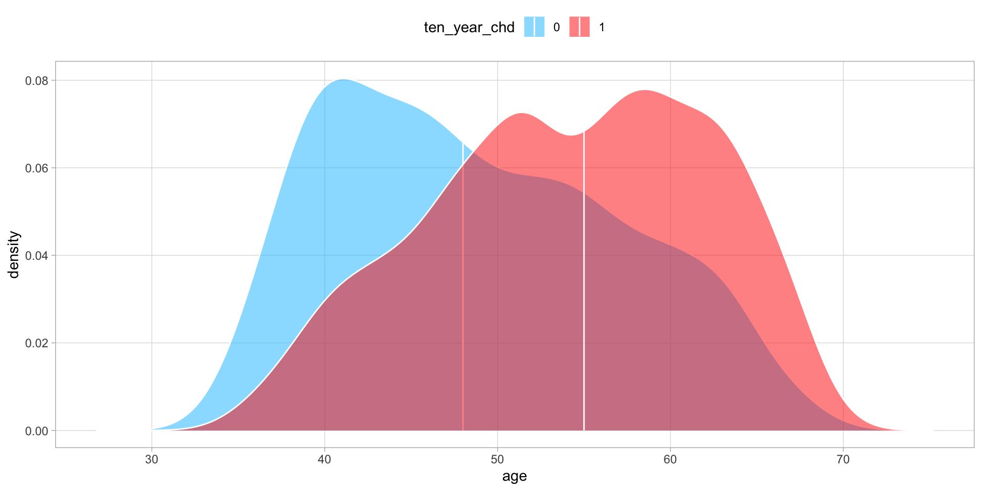
And the effect of age is slightly different for men and women, with men showing higher risk of heart disease at younger ages.

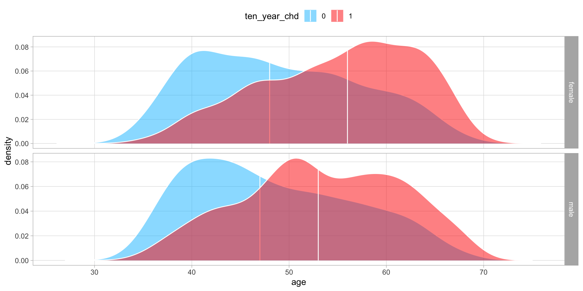
But the most striking observations comes from looking at systolic blood pressure.

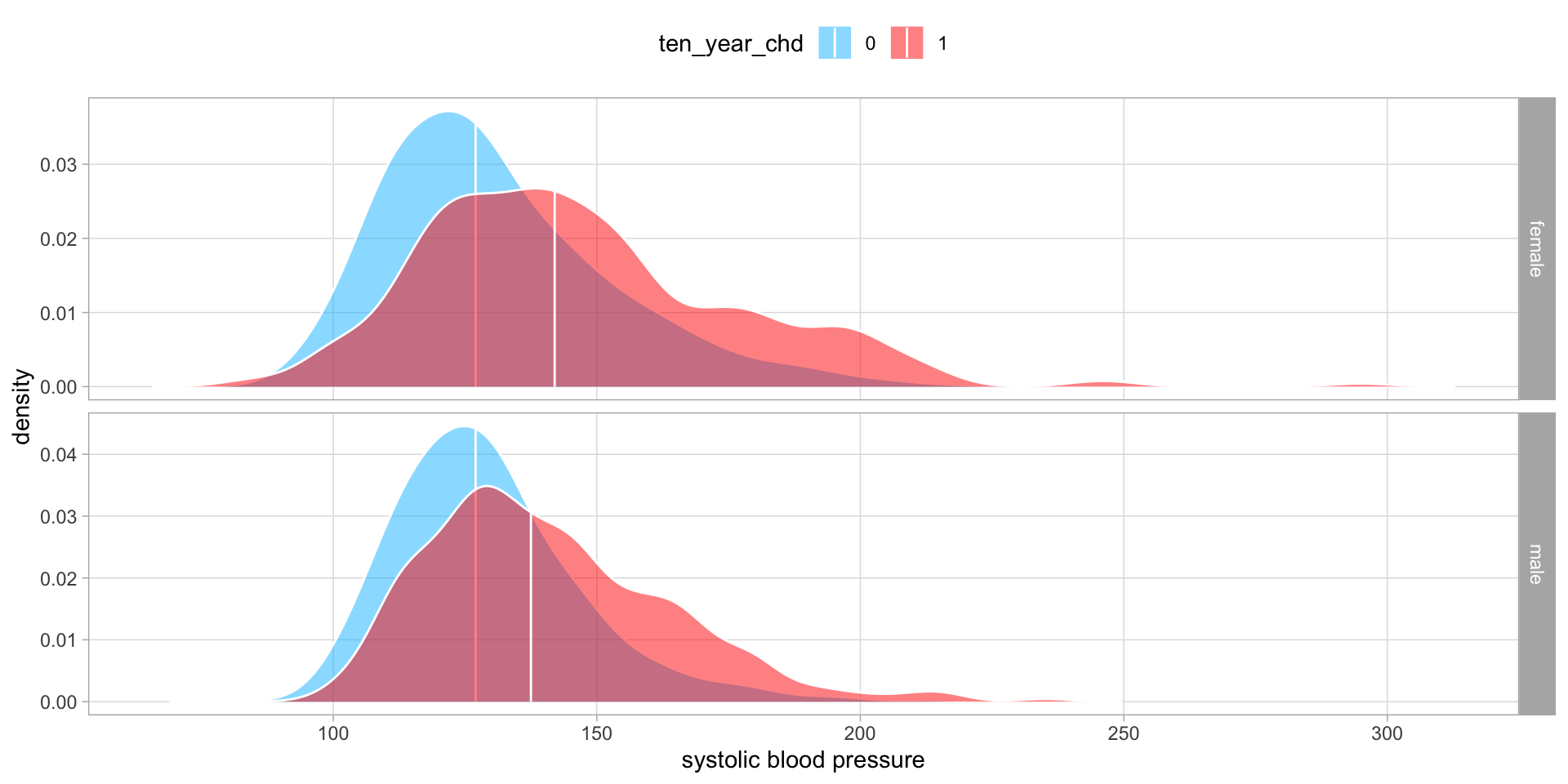
What is the relationship between age, blood pressure, resting heart rate and the onset of future heart disease?

This is the purpose of a model, which we fit to the data to estimate the effect of these features on our outcome.

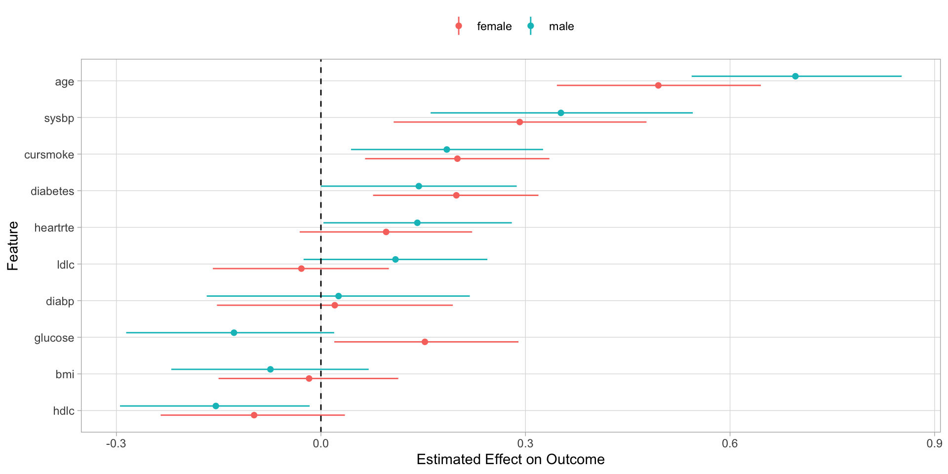
And we end up finding that age, systolic blood pressure, hdlc, and smoking impact an individual’s future risk of heart disease.

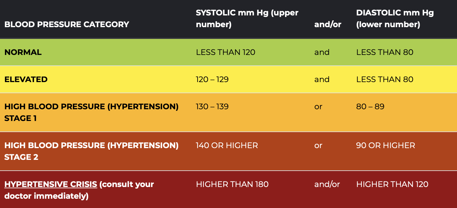
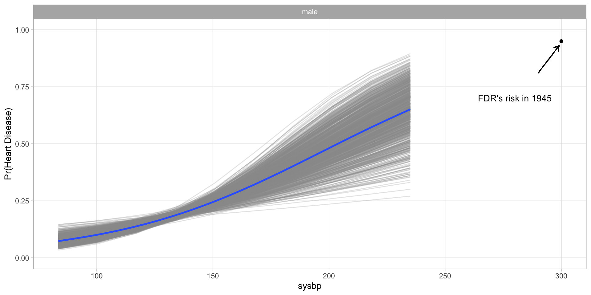
How does blood pressure affect the risk of heart disease?

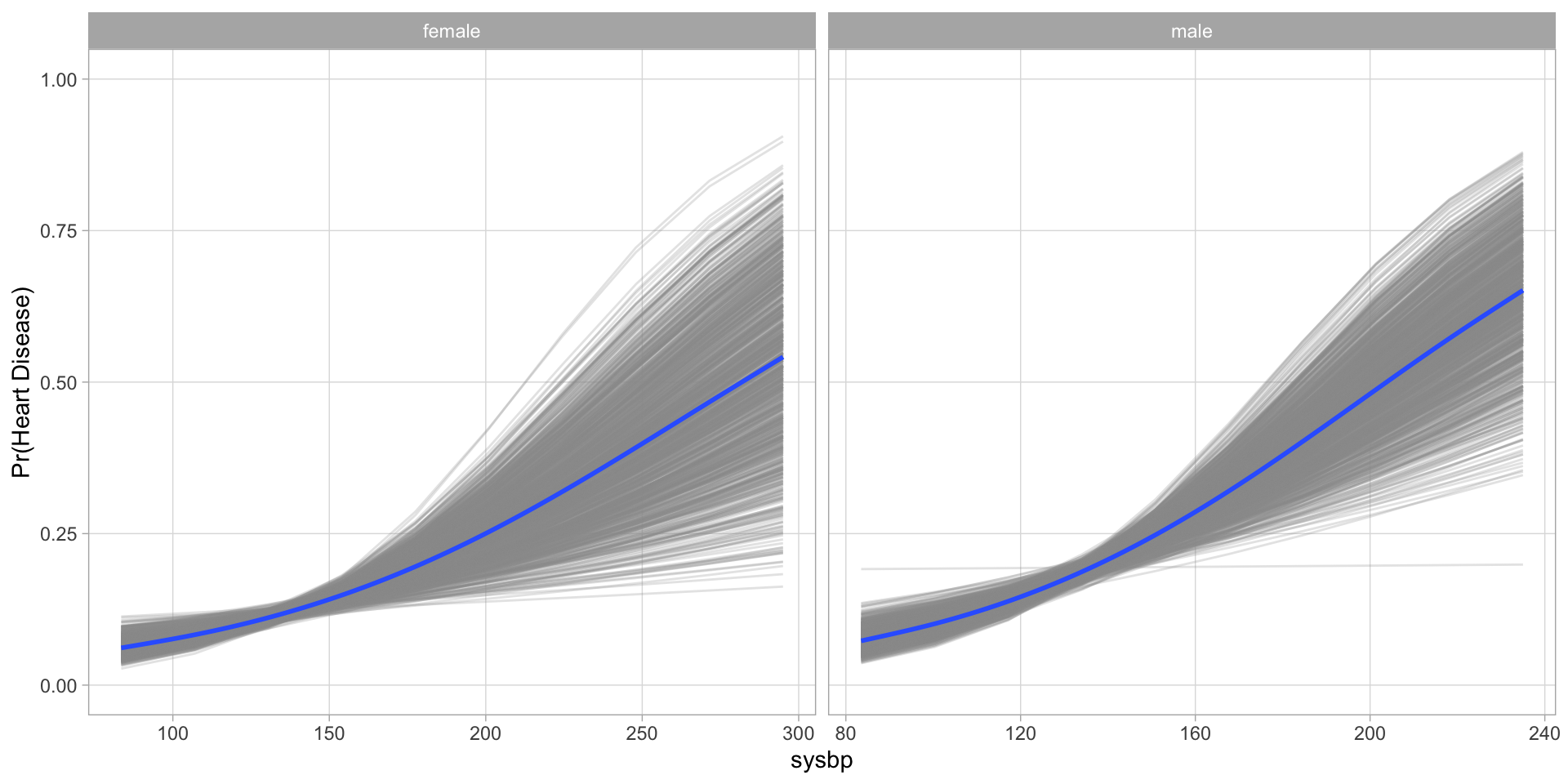
This is what the researchers found in the original Framingham study.

The first major findings from the original cohort were published in 1957, almost a decade after the initial participant was examined.

They found a nearly 4 fold increase in coronary heart disease incidence per 1000 persons among hypertensive participants (≥160/95 mmHg).

If you were wondering what this model would have predicted for FDR based on his blood pressure.

Much of what we know about the causes of heart disease (exercise, diet, smoking) was found in the years to come in the more than 3000 papers published using data from the Framingham Heart Study.

These findings form the basis of the Framingham Risk Score, a simple model for estimating long term risk of cardiovascular disease that is used to this day.

Much of what we know about the causes of heart disease (exercise, diet, smoking) was found in the years to come in the more than 3000 papers published using data from the Framingham Heart Study.

These findings form the basis of the Framingham Risk Score, a simple model for estimating long term risk of cardiovascular disease that is used to this day.

The Framingham study continues; it is now on its third generation of residents, examining the effects of family history and genetics.

Why am I telling you about this?

1. The data you choose to collect, and not collect, is part of the scientific process.

2. All of the technology in the world does not matter if you do not understand your problem and the data and methodology that would help you solve it.

The methods we use to understand something as simple as heart disease are the same ones we use to make predictions for something far more serious: college football.

2) How do you predict football games?

Have you ever looked at pre-game betting lines and win probabilities for football games?

Have you ever wondered how they make these predictions?

Would you have guessed that it had something to do with a quarterback who played in the 1970s?

Virgil Carter was an NFL quarterback who played for the Bears and the Bengals in the 1970s.

While also being a quarterback in the NFL, Virgil Carter earned a Master’s degree from Northwestern and taught statistics and mathematics at Xavier University.

The focus of his research, naturally, was football.

How do you evaluate a football team?

Virgil Carter’s idea was to measure the value of individual plays in terms of expected points.

To illustrate: how many points is each of the following plays worth?

To answer questions like these, Virgil Carter manually collected play-by-play data from the entire 1969 NFL season.

He wanted to calculate the expected value of field position in terms of points, or expected points.

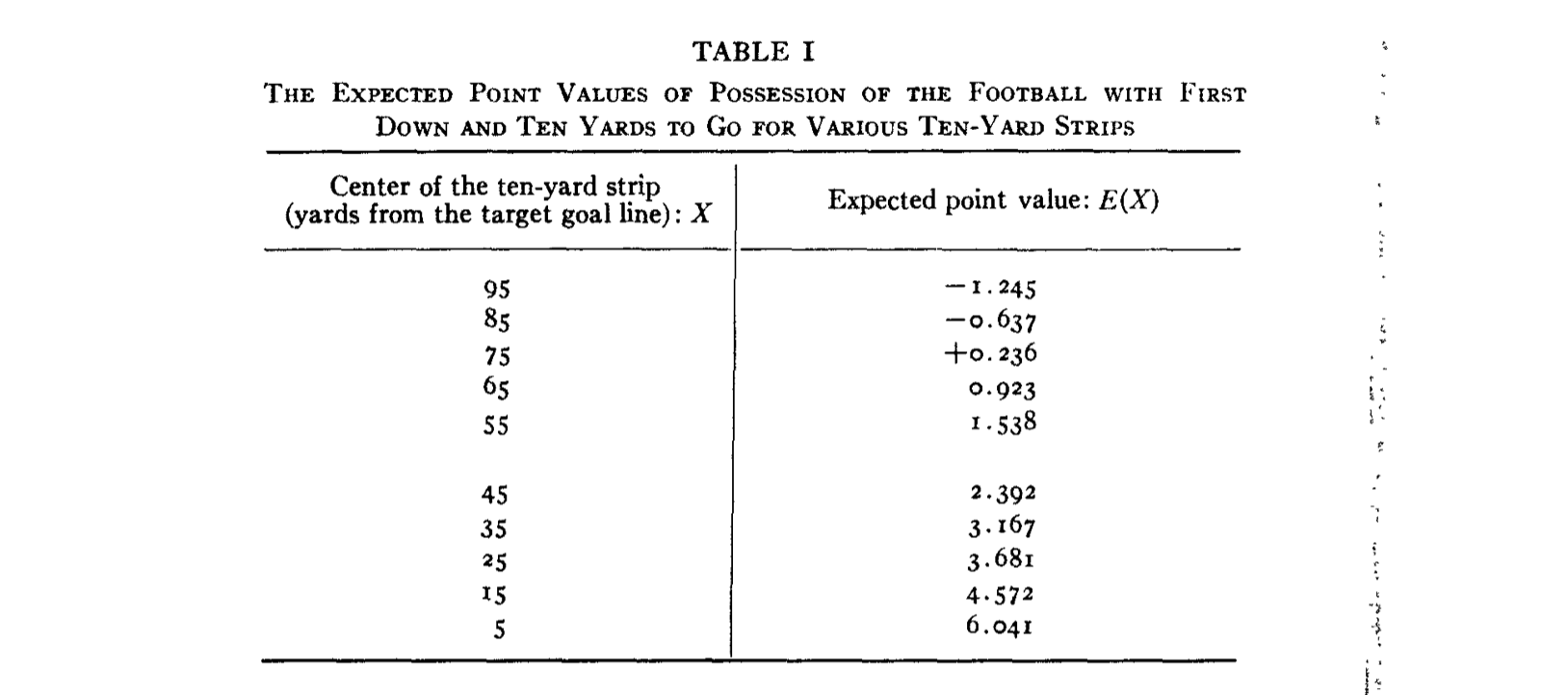
What did he mean by expected points?

Suppose your offense starts a drive on its own 15 yard line. On average, how many points do teams in this situation typically go on to score?

From his calculations: -0.637. Why?

On average, teams starting from their 15 yard line are less likely to score next than their opponents.

But, imagine your offense completes a pass for 10 yards and moves to your 25. Now, your expected points is positive: 0.236. Why?

On average, teams on their own 25 yard line were more likely to score next than their opponents.

That 10 yard pass improved your situation quite a bit, changing your expected points from -0.637 to 0.236.

The play’s expected points added is 0.873.

This is how we measure the value of plays in college football.

Expected Points Before Play: 1.80
Expected Points After Play: 7.00
Expected Points Added: 5.20

Expected Points Before Play: 0.67
Expected Points After Play: 1.80
Expected Points Added: 1.13

Expected Points Before Play: 0.20
Expected Points After Play: -3.25
Expected Points Added: -3.45

Note: these estimates are not based on Virgil Carter’s 1969 NFL season, but my own expected points model trained on all college football plays from 2007-2019.

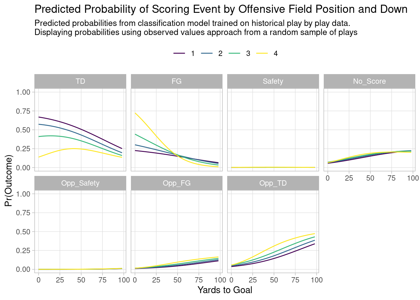
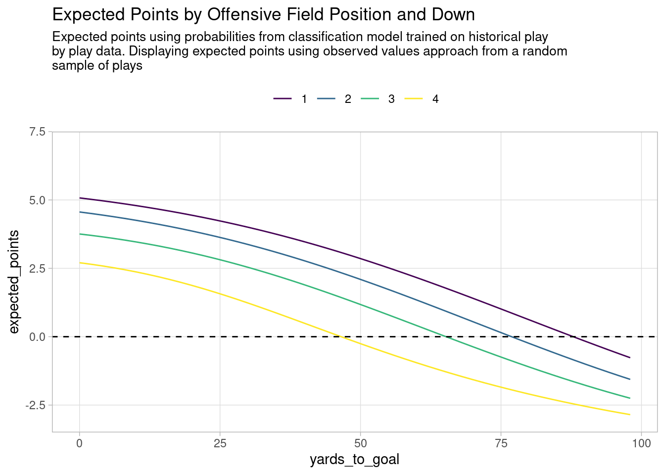
Virgil Carter’s idea forms the basis of modern football analytics and how we evaluate teams and players:

Good offenses generate points in expectation.
Good defenses prevent points in expectation.

We evaluate teams based on plays and their efficiency in terms of expected points.

This turns out to be an effective way to measure a team’s performance for the purpose of predicting games.

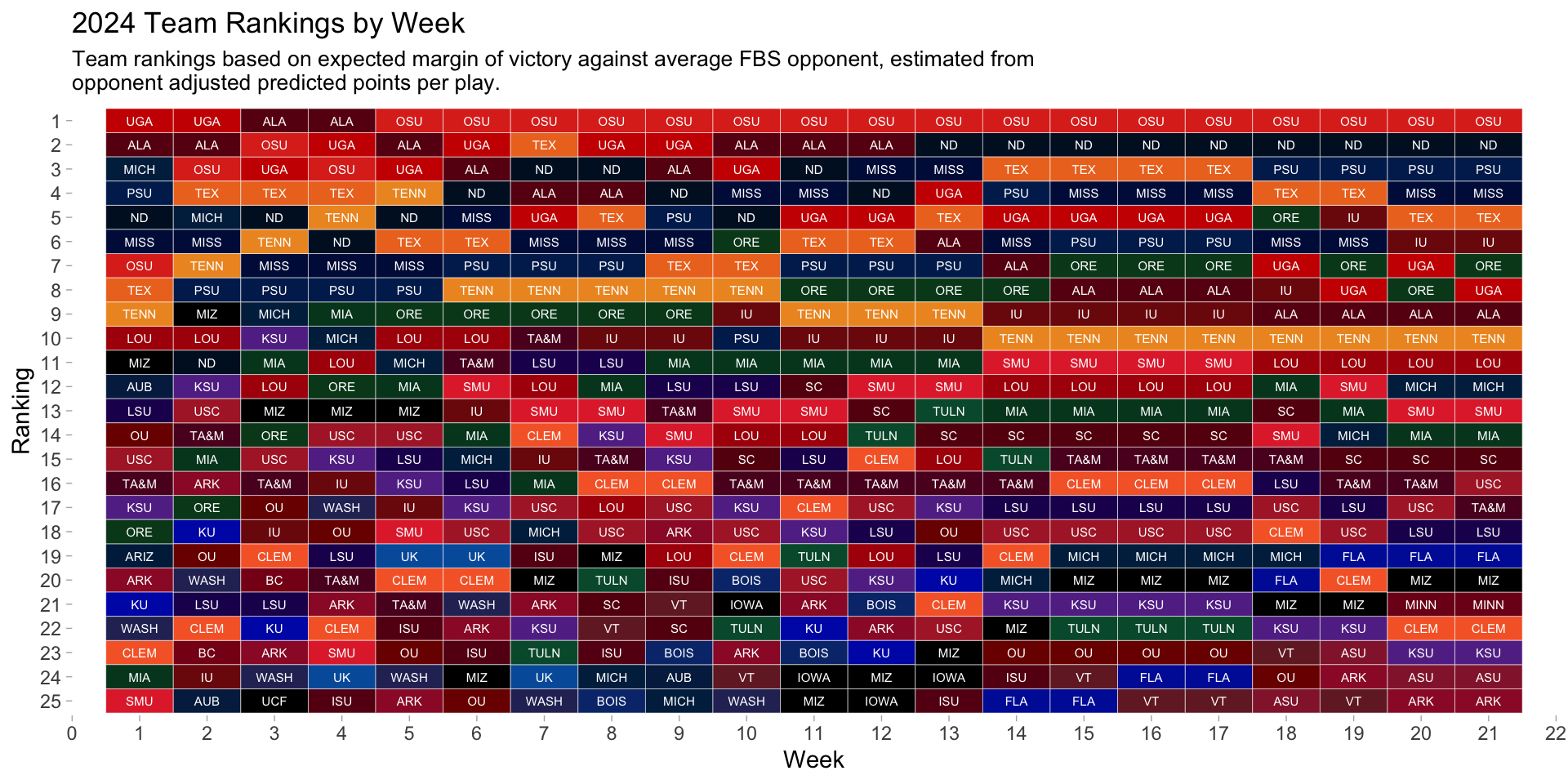
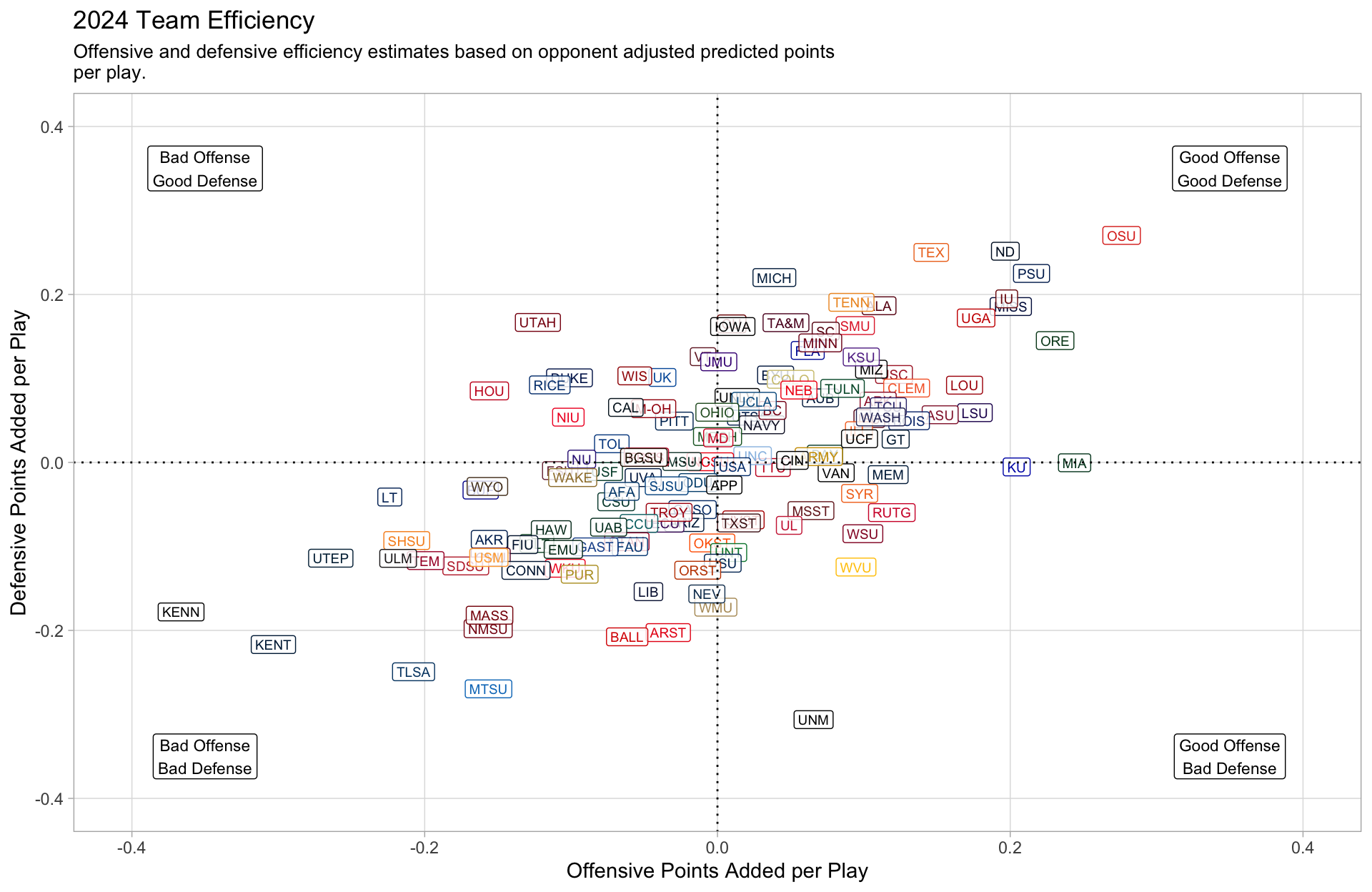
How do you predict college football games?

You measure the efficiency of every team’s offense and defense based on every play that has occurred over the course of a season via expected points.¹

You simultaneously estimate a rating for every team’s offense and defense, conditional on every other team’s offense and defense.²

1. Technically, this is fairly involved and this measurement also includes plays from previous seasons with increasingly less weight assigned to them. A full discussion of this is done would take some time; I would be happy to talk about it in exhausting detail with you later.

2. This is also fairly involved but can be accomplished via a ridge regression; again, I would be happy to talk about it in exhausting detail with you later.

For example, this is where teams were rated in terms of efficiency on the eve of the College Football Playoff Semi Finals.

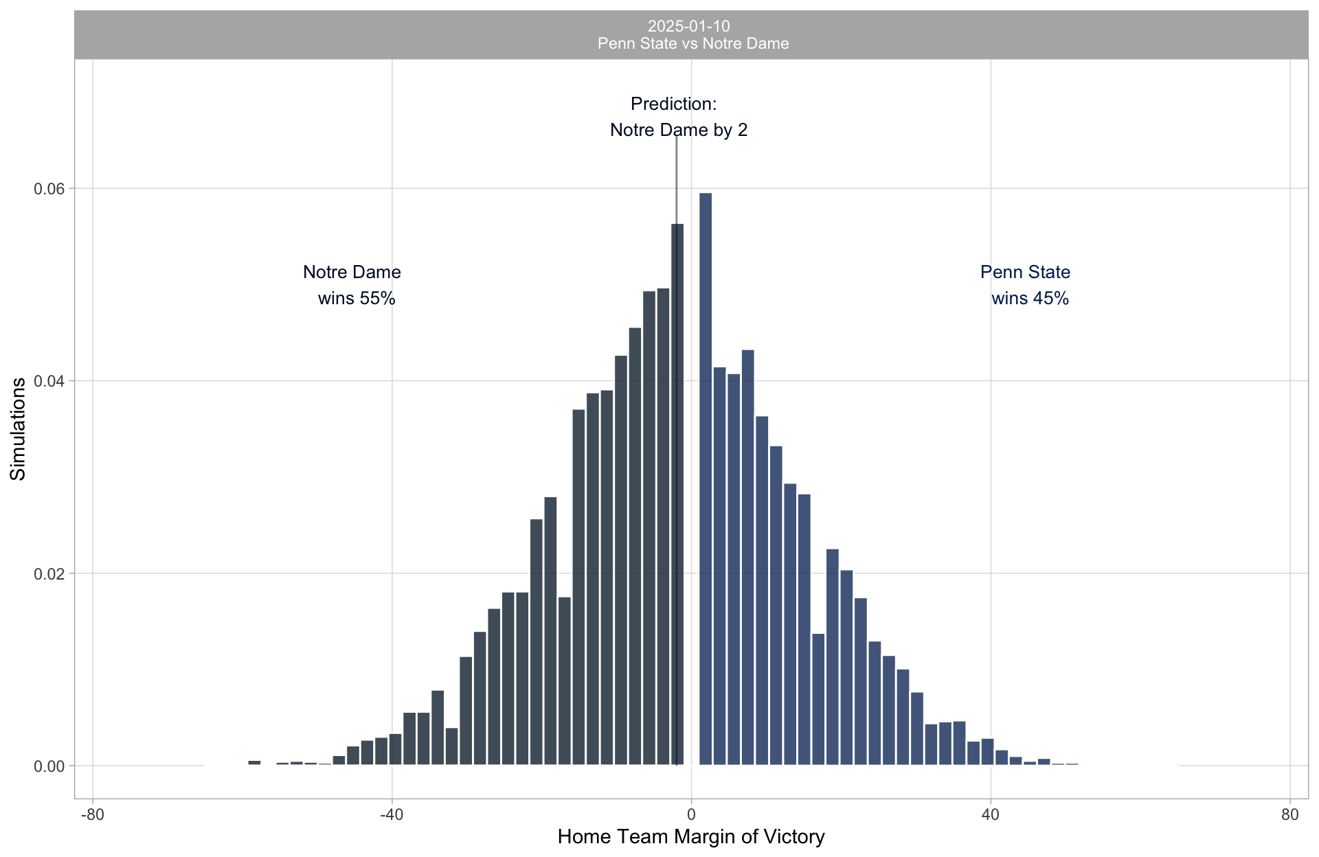
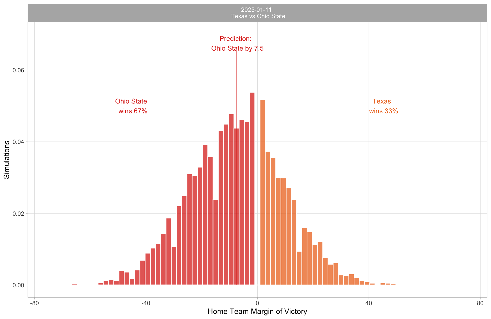
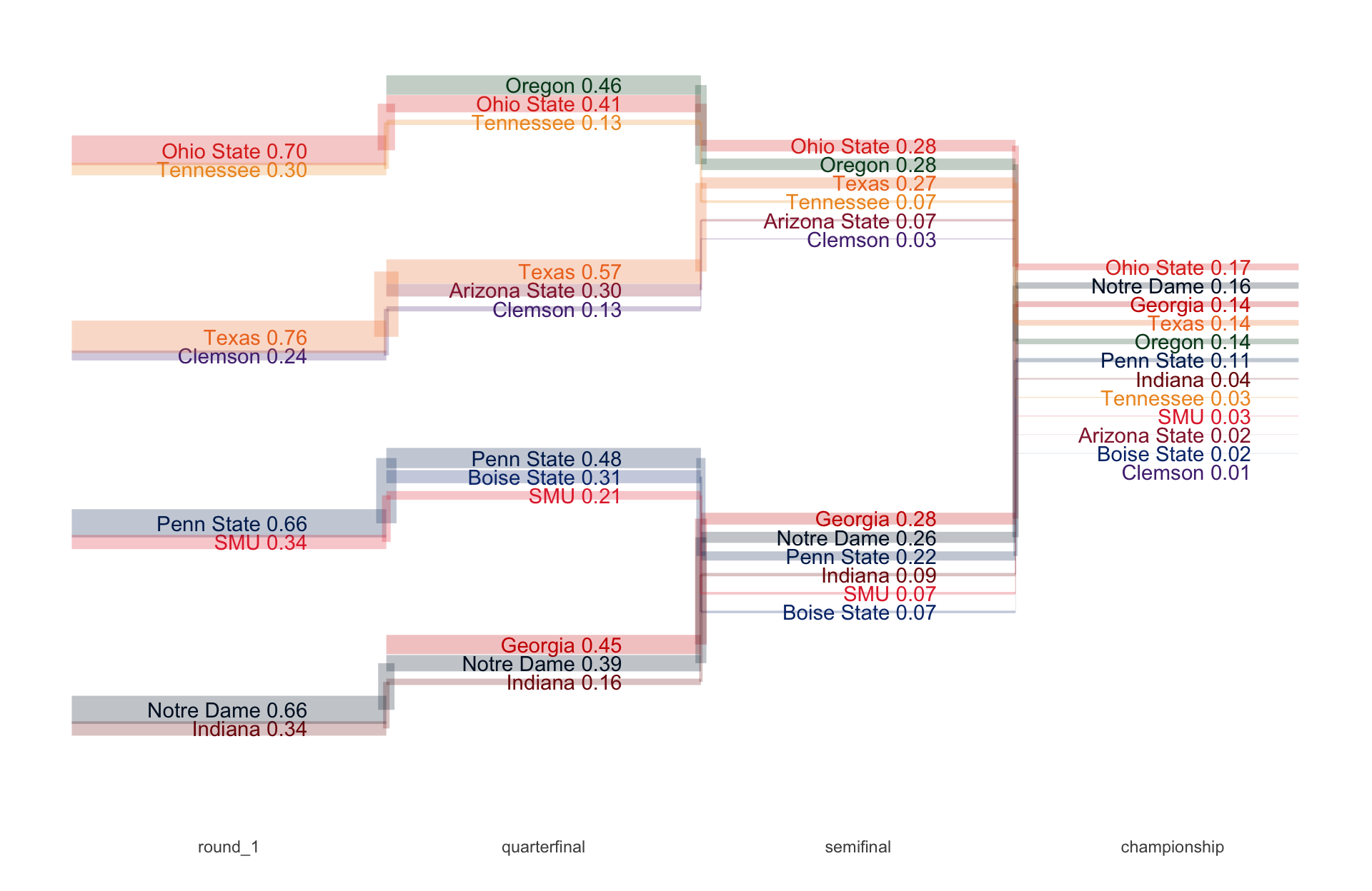
You then use these estimates of team efficiency to simulate the outcome of games.

For example, these are the simulations for the semi final games.

Is that really how they do it?

I was working on my own series of models for evaluating teams and eventually decided to compare my work to that of ESPN and Vegas.

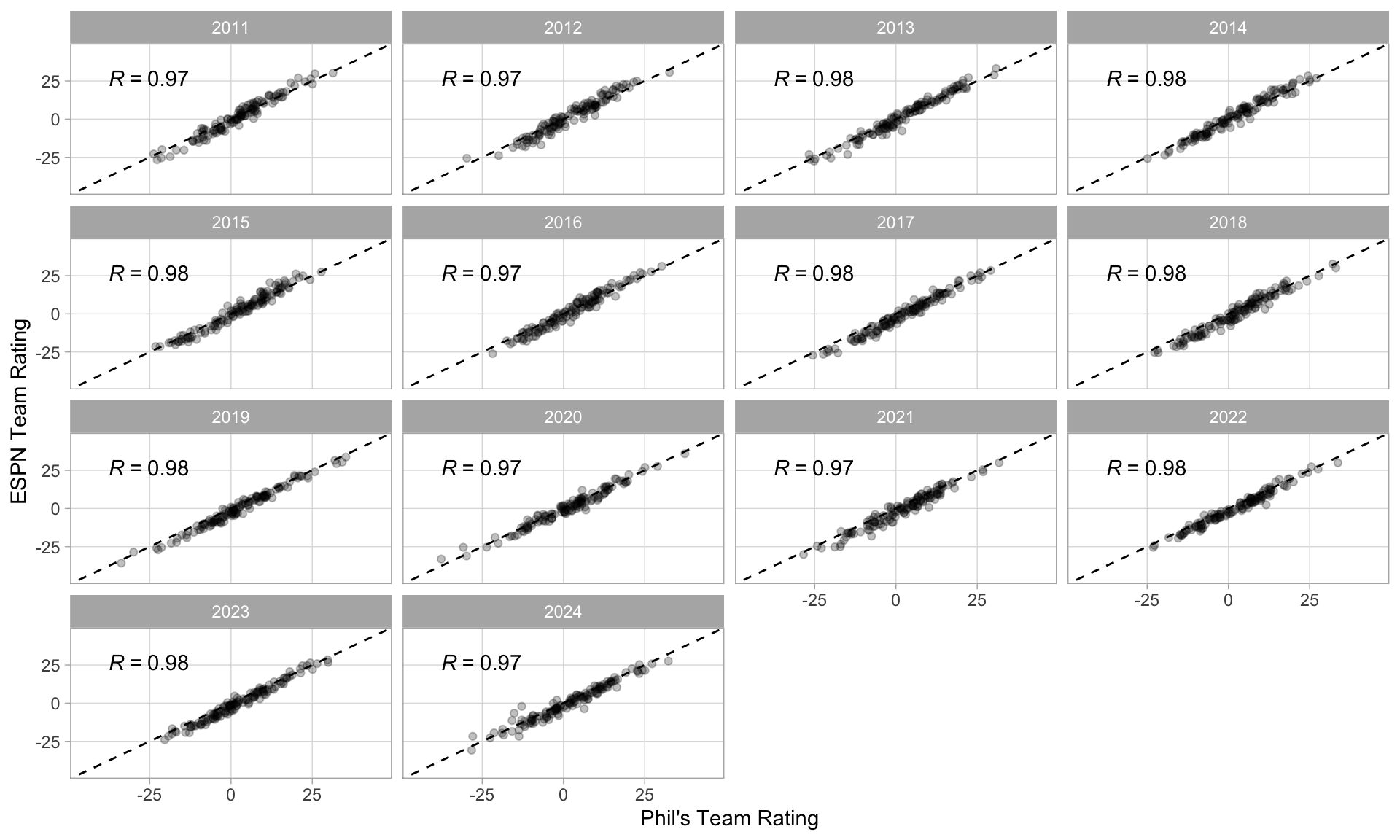
My end of year team ratings compared to the ESPN college football power index.

My spread vs opening spreads from providers throughout the 2024 season.

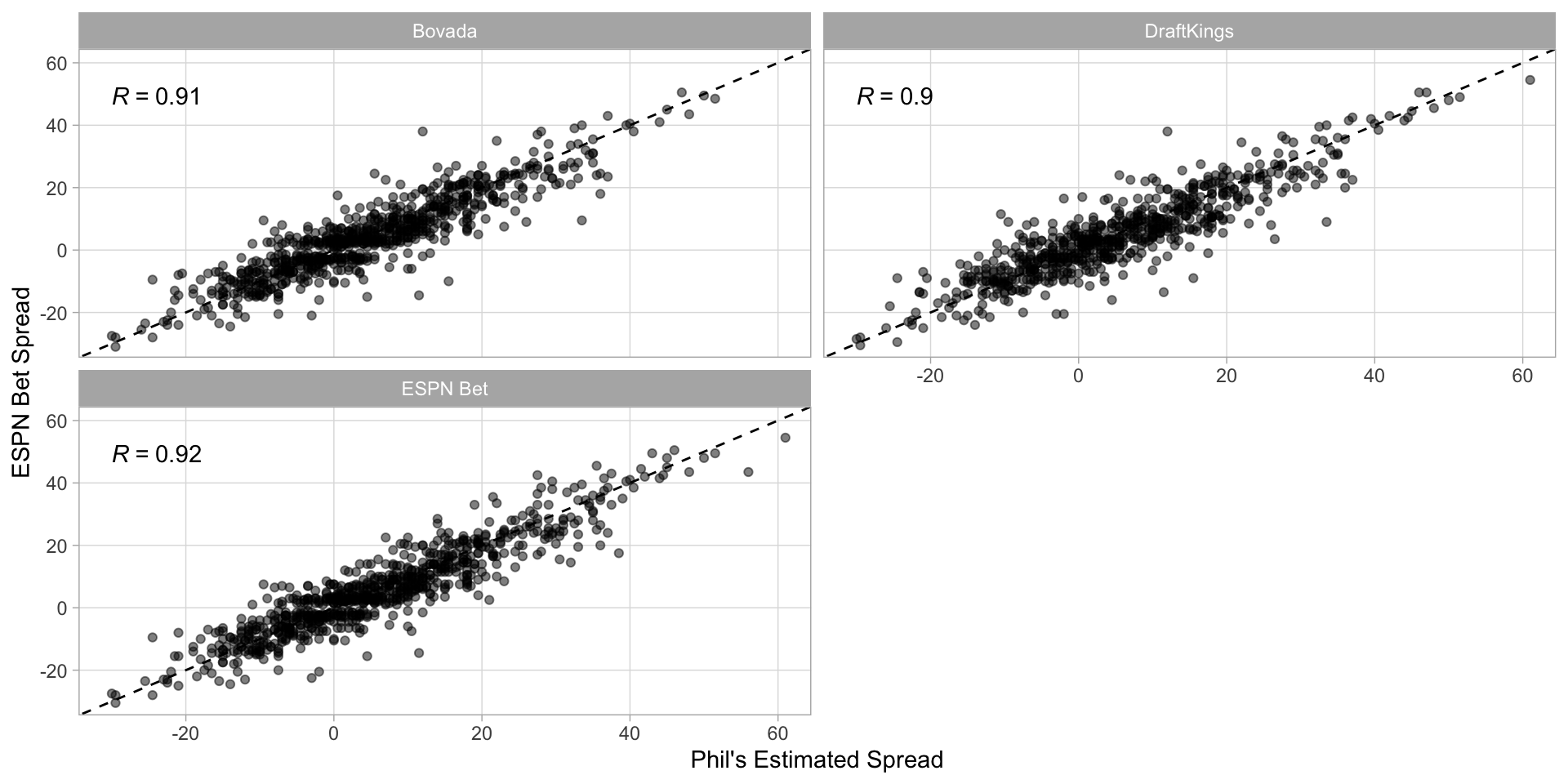
Betting lines for individual games are a little bit harder to crack; they are surely accounting for things that I (currently) am not, such as rest/injuries/travel.

However, my model performs about as well in predicting games.

season	model	games	record	accuracy
2024	ESPN Bet	897	664-233	0.740
2024	Phil	904	660-244	0.730
2024	DraftKings	810	586-224	0.723
2024	Bovada	801	572-229	0.714

My record against the spread for each provider.

season	provider	games	record	accuracy
2024	Bovada	801	417-383	0.521
2024	DraftKings	810	425-372	0.533
2024	ESPN Bet	897	464-433	0.517

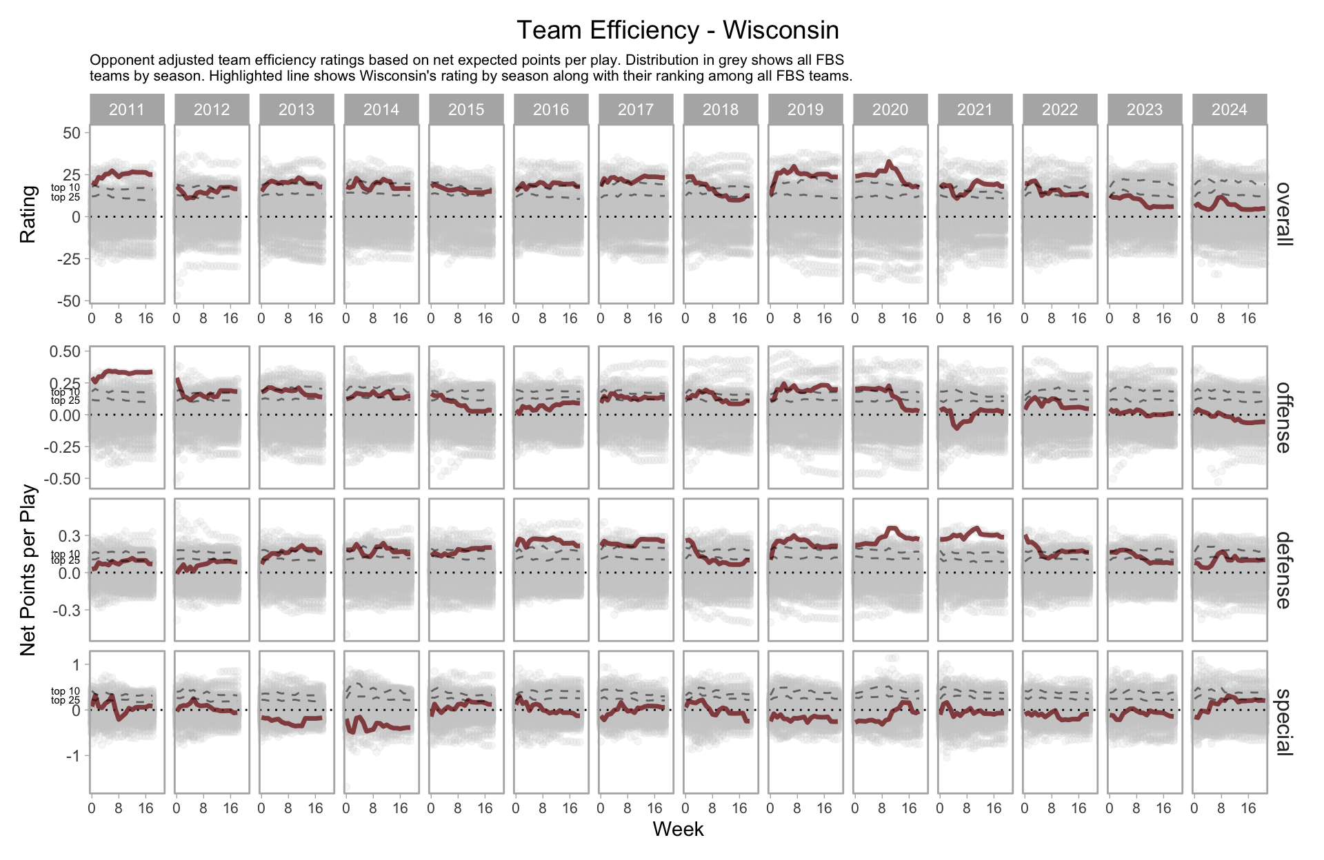
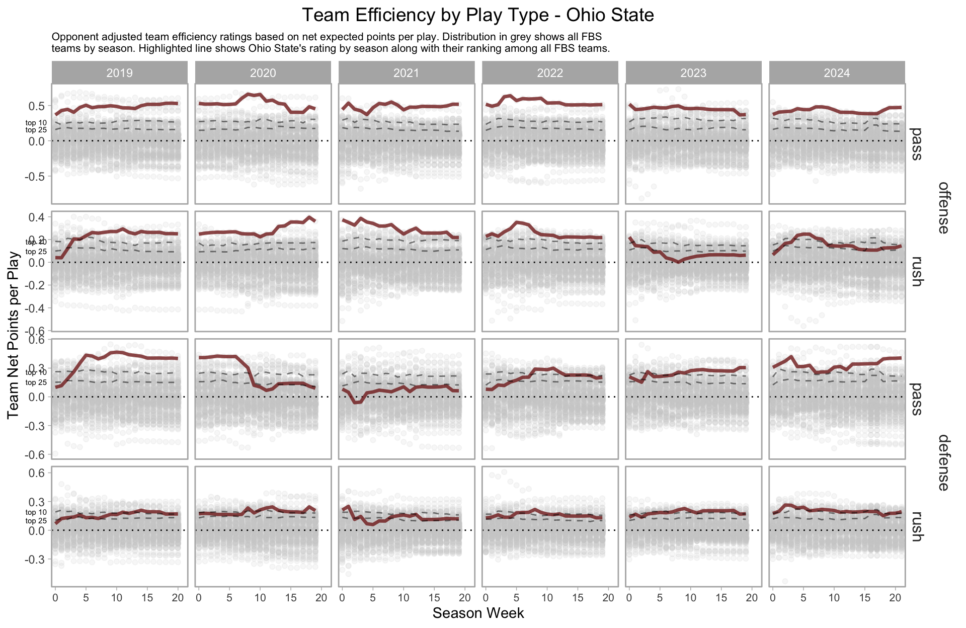
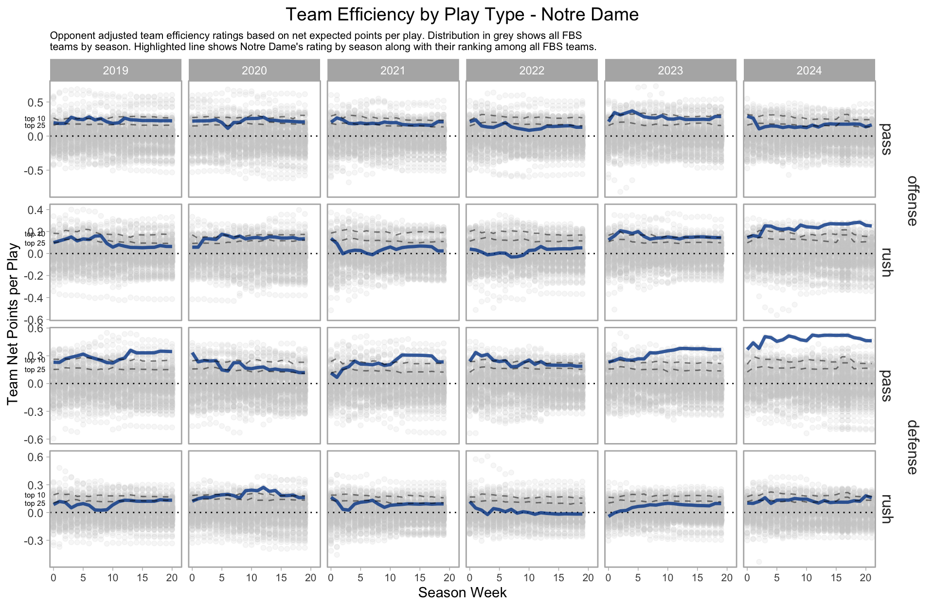
Beyond prediction, using a model allows us to measure and monitor a team’s performance based on their underlying play, not just their record.

For instance, Wisconsin’s estimated performance by week since 2019.

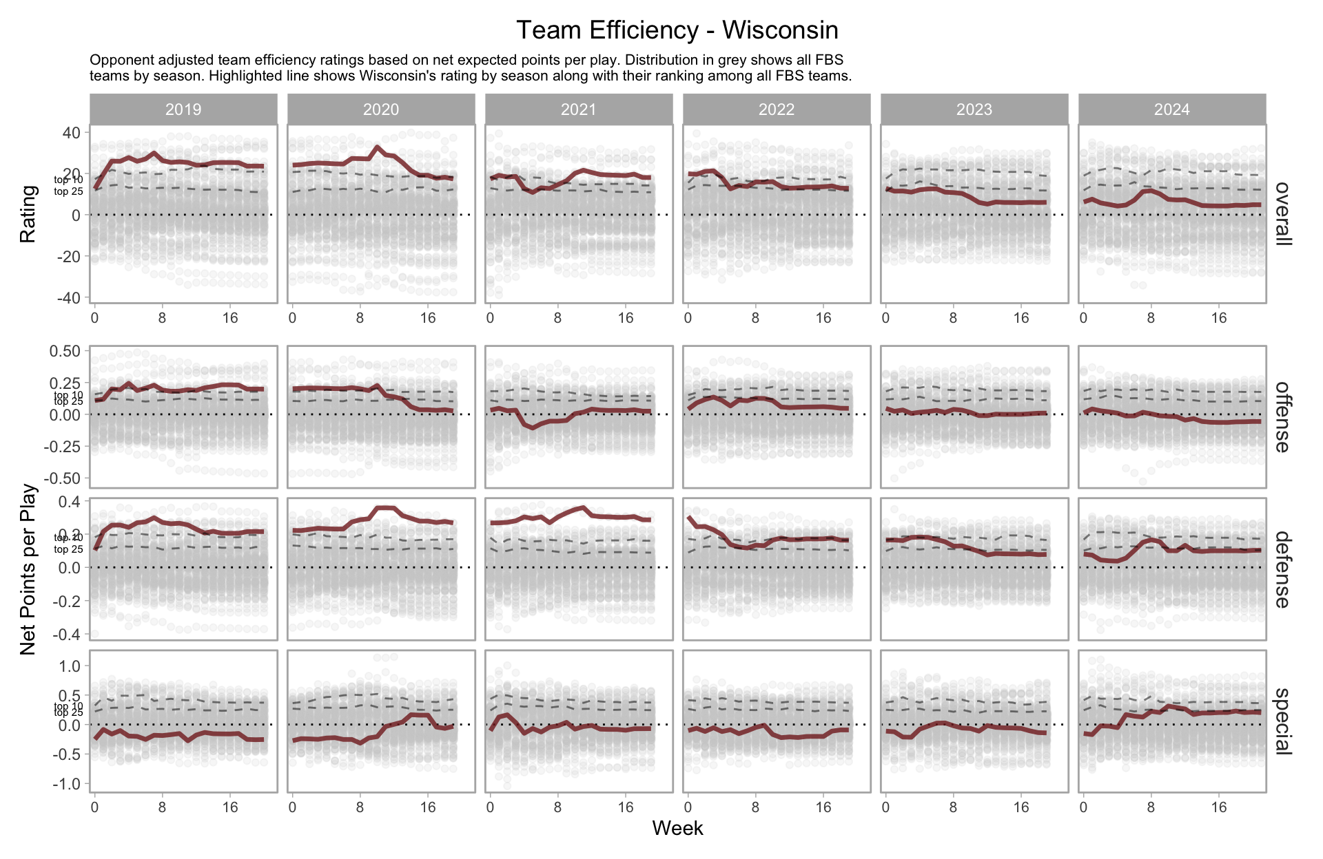
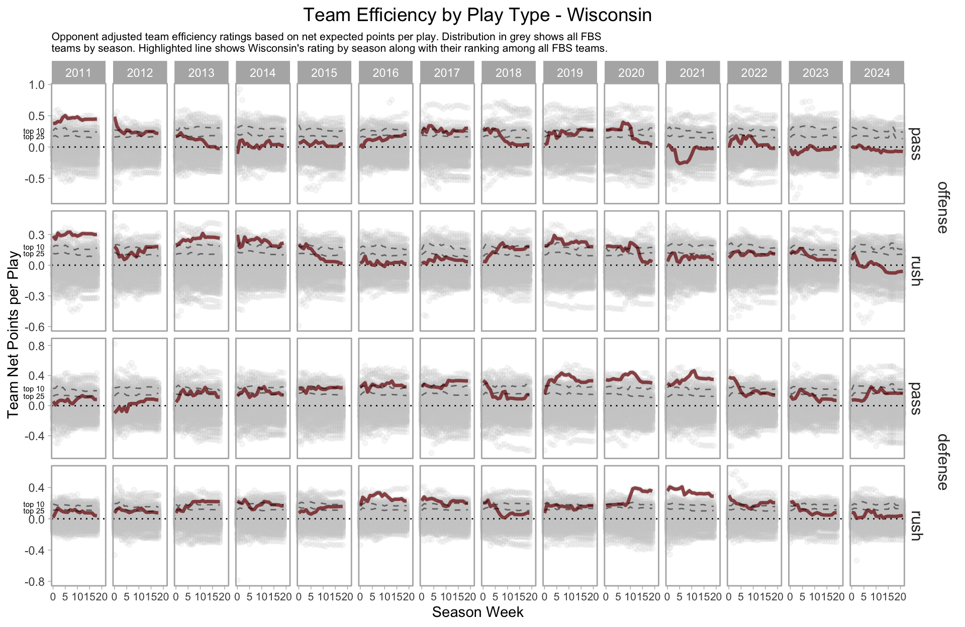
We can break this down further based on pass/rush, which paints a pretty grim picture for Wisconsin’s offense.

Why am I telling you about this?

1. Models are about more than just prediction; they enable us to make sense of patterns in data and measure things we care about.

2. The best work and the best predictions tend to come from really trying to understand the thing you are predicting.

Bonus Round

Predicting the CFB Playoff

How do you predict the college football playoff?

You use your measures of team performance to simulate how the playoff might unfold. You do this thousands of times.

I ran my simulations on the eve of the playoff.

I will admit, I was suspicious of the results and my own model. But this was the result.

2024 College Football Playoff Simulations
Results based on 10,000 simulations from team efficiency model
team	team rating		win probability
	offense	defense	Round 1	Quarterfinal	Semi-Final	Championship
Ohio State	0.219	0.245	0.696	0.409	0.279	0.166
Notre Dame	0.215	0.257	0.658	0.388	0.265	0.158
Georgia	0.209	0.142	✓	0.454	0.284	0.143
Texas	0.133	0.290	0.759	0.570	0.270	0.143
Oregon	0.230	0.155	✓	0.458	0.276	0.138
Penn State	0.219	0.198	0.662	0.478	0.223	0.106
Indiana	0.192	0.198	0.342	0.158	0.088	0.042
Tennessee	0.092	0.226	0.304	0.133	0.073	0.031
SMU	0.132	0.165	0.338	0.211	0.072	0.027
Arizona State	0.152	0.054	✓	0.302	0.068	0.018
Boise State	0.135	0.047	✓	0.311	0.069	0.018
Clemson	0.130	0.120	0.241	0.128	0.034	0.010

My model has been stubborn that Ohio State is the best team in college football since the end of September.

It has only grown more confident about Ohio State after each round.

2024 College Football Playoff Simulations
Results based on 10,000 simulations from team efficiency model
team	team rating		win probability
	offense	defense	Round 1	Quarterfinal	Semi-Final	Championship
Ohio State	0.219	0.245	0.696	0.409	0.279	0.166
Notre Dame	0.215	0.257	0.658	0.388	0.265	0.158
Georgia	0.209	0.142	✓	0.454	0.284	0.143
Texas	0.133	0.290	0.759	0.570	0.270	0.143
Oregon	0.230	0.155	✓	0.458	0.276	0.138
Penn State	0.219	0.198	0.662	0.478	0.223	0.106
Indiana	0.192	0.198	0.342	0.158	0.088	0.042
Tennessee	0.092	0.226	0.304	0.133	0.073	0.031
SMU	0.132	0.165	0.338	0.211	0.072	0.027
Arizona State	0.152	0.054	✓	0.302	0.068	0.018
Boise State	0.135	0.047	✓	0.311	0.069	0.018
Clemson	0.130	0.120	0.241	0.128	0.034	0.010

2024 College Football Playoff Simulations
Results based on 10,000 simulations from team efficiency model
team	team rating		win probability
	offense	defense	Round 1	Quarterfinal	Semi-Final	Championship
Ohio State	0.253	0.248	✓	0.642	0.439	0.267
Notre Dame	0.220	0.257	✓	0.599	0.368	0.198
Penn State	0.208	0.232	✓	0.766	0.367	0.167
Texas	0.150	0.270	✓	0.746	0.310	0.155
Oregon	0.234	0.157	✓	0.358	0.207	0.099
Georgia	0.204	0.144	✓	0.401	0.219	0.095
Boise State	0.135	0.045	✓	0.234	0.047	0.010
Arizona State	0.151	0.052	✓	0.254	0.043	0.009

2024 College Football Playoff Simulations
Results based on 10,000 simulations from team efficiency model
team	team rating		win probability
	offense	defense	Round 1	Quarterfinal	Semi-Final	Championship
Ohio State	0.272	0.261	✓	✓	0.666	0.407
Notre Dame	0.186	0.264	✓	✓	0.546	0.254
Penn State	0.203	0.236	✓	✓	0.454	0.184
Texas	0.155	0.257	✓	✓	0.334	0.154

So far, the playoff has gone almost exactly to script.

season	week	home	away	Pr(Home Win)	prediction	actual	Correct?
2024	18	Notre Dame	Indiana	0.678	Notre Dame by 7.5	Notre Dame by 10	✓
2024	18	Penn State	SMU	0.667	Penn State by 7.5	Penn State by 28	✓
2024	18	Texas	Clemson	0.752	Texas by 12	Texas by 14	✓
2024	18	Ohio State	Tennessee	0.693	Ohio State by 8.5	Ohio State by 25	✓
2024	20	Boise State	Penn State	0.233	Penn State by 12	Penn State by 17	✓
2024	20	Arizona State	Texas	0.261	Texas by 10.5	Texas by 8	✓
2024	20	Oregon	Ohio State	0.312	Ohio State by 8.5	Ohio State by 20	✓
2024	20	Georgia	Notre Dame	0.404	Notre Dame by 4.5	Notre Dame by 13	✓
2024	21	Penn State	Notre Dame	0.462	Notre Dame by 1.5	Notre Dame by 3	✓
2024	21	Texas	Ohio State	0.320	Ohio State by 7.5	Ohio State by 14	✓

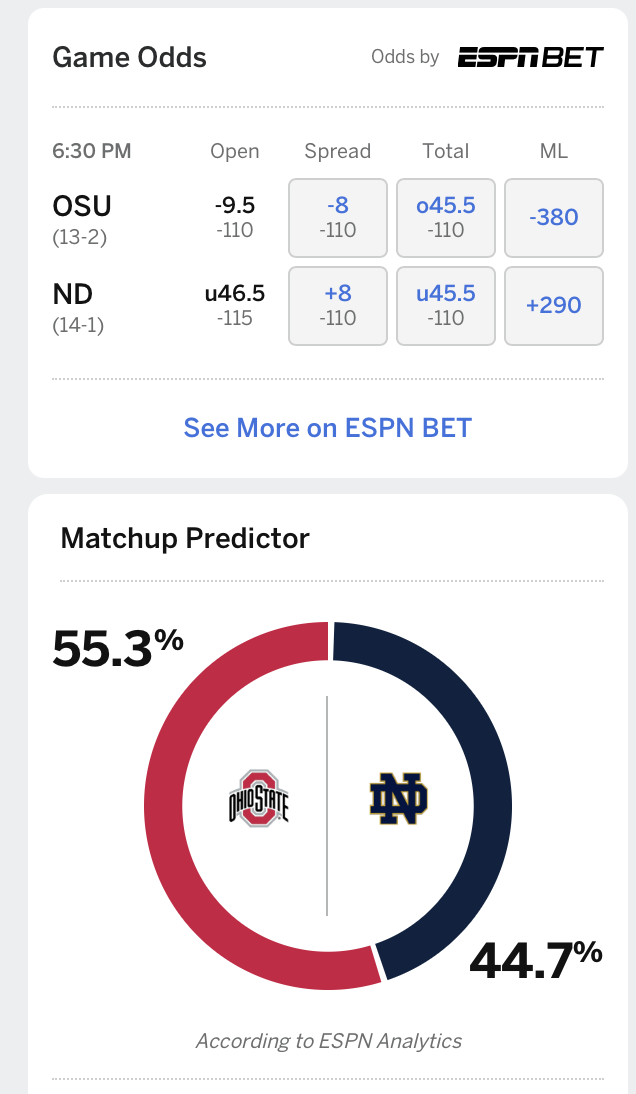
Which brings us to the national championship, which for my money is between the two best teams in college football.

Season	Team	Pass Offense	Run Offense	Pass Defense	Run Defense
2024	Ohio State	0.473 (1)	0.145 (15)	0.406 (2)	0.194 (7)
2024	Notre Dame	0.164 (21)	0.251 (2)	0.462 (1)	0.159 (18)

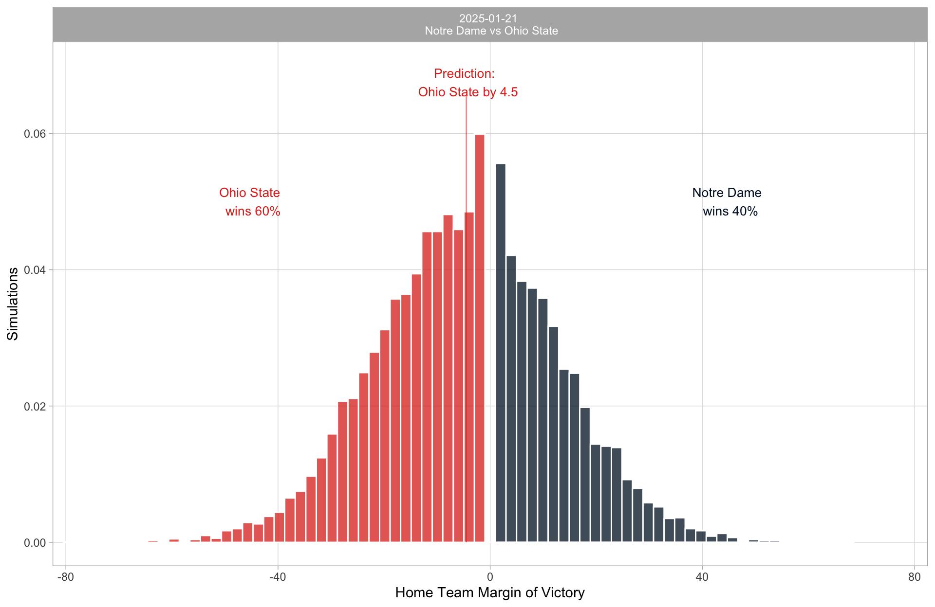
What’s the prediction?

2024 College Football Playoff Simulations
Results based on 10,000 simulations from team efficiency model
team	team rating		win probability
	offense	defense	Round 1	Quarterfinal	Semi-Final	Championship
Ohio State	0.276	0.270	✓	✓	✓	0.604
Notre Dame	0.197	0.251	✓	✓	✓	0.396

Ireland wins but Krum gets the snitch

Ohio State wins but doesn’t cover. Ohio State by 4.5.

wrapping up

The value of data science is simply that of science - it is the process by which we understand the world around us.

It allows us to discover cause and effect; it allows us to measure things we care about. It helps us understand the data we have and the data that we don’t.

To recap:

1. The data you choose to collect, and not collect, is part of the scientific process.

2. All of the technology in the world does not matter if you do not understand your problem and the data and methodology that would help you solve it.

3. Models are about more than just prediction; they enable us to make sense of patterns in data and measure things we care about.

4. The best work and the best predictions tend to come from really trying to understand the thing you are predicting.

one final thought

There is no easy button; there is no tool that you can buy and start solving all of your problems.

The value in (data) science usually doesn’t come from algorithms, tools, platforms.

The value in (data) science is usually from the creativity/dedication/passion of asking questions and caring about finding the answer.

I don’t think data science is electricity or data the new oil. I think it’s something much simpler.

(Data) science is like farming.

It’s slow and difficult and takes a lot of patience.

But if you work at it and make an effort everyday, you will produce something valuable in the end.

thanks for listening

references

1. Mahmood, Syed S., et al. “The Framingham Heart Study and the epidemiology of cardiovascular disease: a historical perspective.” The lancet 383.9921 (2014): 999-1008.

2. Dawber, Thomas R., Gilcin F. Meadors, and Felix E. Moore Jr. “Epidemiological approaches to heart disease: the Framingham Study.” American Journal of Public Health and the Nations Health 41.3 (1951): 279-286.

3. Epidemiological Background and Design: The Framingham Heart Study

4. Carter, Virgil, and Robert E. Machol. “Operations research on football.” Operations Research 19.2 (1971): 541-544.